Programmatic Sol LeWitt Wall Drawing

I visited MASS MoCA with some friends recently. There was a whole building there filled with the work of Sol LeWitt, a contemporary artist famous for minimalist geometric art. We spent a while looking at Wall Drawing #797.

Helen Harrison

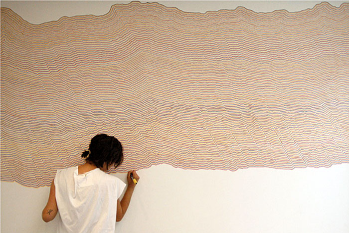
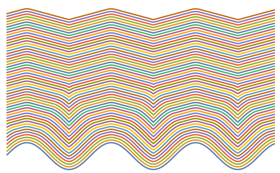
This drawing was made in an interesting way. One person drew a starting wavy line at the top. Then artists took turns following the bottom of the line with another line. This was repeated for the whole wall. The result has some complicated behavior. Concave parts produced ridges propagating downward and combining into larger ridges. It reminded us of caustic shapes produced by the complex surface of disturbed water. Phil pointed out that the connection with waves isn't an accident, since this procedure effectively applies Huygens' Principle. He blogged about this too, but my post is better.

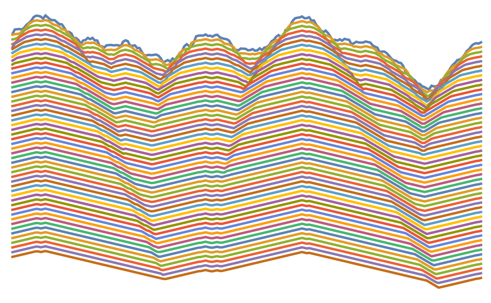
We all thought it would be cool to reproduce this idea in a computer. I found a way to do it with a few lines of Mathematica.

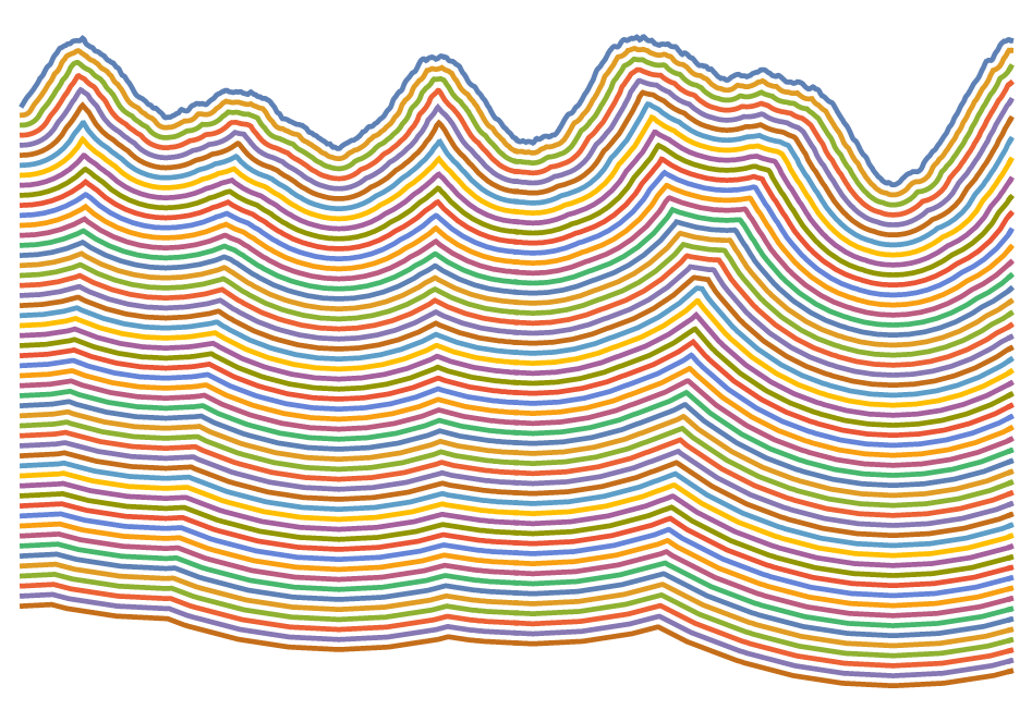
Not a perfect match, but it has most of the features we noticed. The heart of it is the overloaded function, requiredY. The points that make up the lines are confined to discrete positiosn in x. With two arguments, it finds the new y value required to put a new point at in the column at index i based on being a distance r from the last point in the row at index j. With one argument, it finds the minimum y required by all other rows. Maybe that makes sense. The rest of the code is just defining the starting curve, repeatedly applying the function that generates a new line, and displaying the results.

xs = Range[200];
ys = 10 + 5 (Sin[xs/10.] + Sin[xs/6.] + Sin[xs/16.]) +
   Last /@ Normal[
      RandomFunction[WienerProcess[0, .75], {0, 199, 1}]][[1]];
next[xs_, ys_, r_] := Module[{requiredY, newYs},
  requiredY[i_, j_] := ys[[j]] - Sqrt[r^2 - Abs[i - j]^2];
  requiredY[i_] :=
   Min[requiredY[i, #] & /@ Range[Max[i - r, 1], Min[i + r, 200]]];
  newYs = requiredY /@ xs;
  newYs
  ]
ListPlot[NestList[next[xs, #, 2] &, ys, 50], Joined -> True,
 Axes -> False, PlotStyle -> {Thickness[0.005]}]