Solving the Brachistochrone with PyTorch

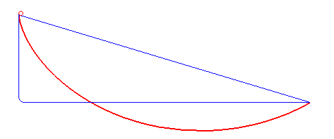
The brachistochrone problem is simple to explain. Imagine a bead which is free to slide on a wire. What shape of wire will get the bead from point A to point B in the shortest time? If you're wondering about the name, "brachistochrone" apparently means "shortest time" in Ancient Greek. Makes sense. The image below shows the optimal path in red, along with some slower paths in blue.

This was inspired by Declan, who was using this problem to learn about genetic algorithms. To quote him, "The genetic optimization algorithm may be the greatest concept to ever emerge from the mind of man." A bit dramatic, I think.

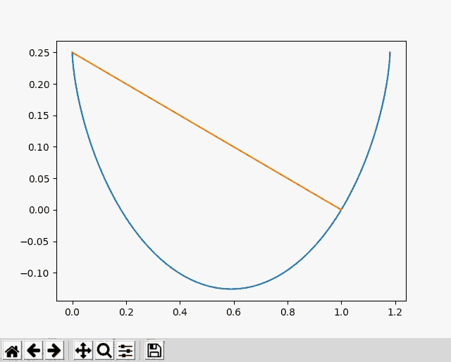
The problem can be solved with calculus, but I decided to approach this problem with gradient descent using PyTorch. It seemed like a natural solution, and a good way to learn about Torch. The image below shows my optimization approaching the shape of the known cycloid solution in blue.

I divided the wire into segments with heights \(y_i\) and calculated the speed at each segment using the height difference from the starting point. Then I found the length of the segments using the height differences between points. I calculated the time to reach each point, \(t_i\), by integrating the segment length divided by the speeds. Finally, I used automatic differentiation to find the derivatives \(\frac{dt_i}{dy_j}\) and used gradient descent to minimize the time to reach the final point, \(t_{last}\).

import torch
import numpy as np
import matplotlib.pyplot as plt
from scipy import optimize

starting_y = 0.25 # y position of the beginning of the wire, end always at 0
xs = torch.linspace(0,1,25) # evenly spaced points in x, from 0 to 1
ys = torch.linspace(starting_y,0,25, requires_grad=True) # start with a straight line connecting start to end

# the physics
def times(ys): # calculate the time to get to each point
	vs = torch.sqrt(starting_y - ys) # find velocity based on height
	dys = ys[1:] - ys[:-1] # find y difference
	dx = xs[1]-xs[0] # find x  difference
	lengths = torch.sqrt(dx.pow(2) + dys.pow(2)) # calculate arc length
	return torch.cumsum((2./(vs[:-1]+vs[1:])) * lengths, dim=0) # integrate to find time to each point using midpoint velocity


fig = plt.figure()
ax = fig.add_subplot(111)

# solving for the cycloid solution
def func(theta):
	return (1.-np.cos(theta)) / (theta - np.sin(theta)) - .25

theta = optimize.brentq(func, 0.01, 2*np.pi)

# parameterized cycloid solution
r = 1 / (theta - np.sin(theta))
ts = np.linspace(0,2 * np.pi,100)
sol_xs = r * (ts-np.sin(ts))
sol_ys = starting_y - r * (1-np.cos(ts))

ax.plot(sol_xs, sol_ys)

li, = ax.plot(xs.numpy(), ys.detach().numpy())

fig.canvas.draw()
plt.show(block=False)

# a pause
raw_input()

# gradient descent
lr = 0.005 # learning rate
for i in range(2000):
	ts = times(ys) # get the times to get to each point
	t = ts[-1] # the time to get to the final point
	t.backward() # back propagate to find gradients
	grads = ys.grad # hold on to the gradient

	# update plots
	li.set_xdata(xs.numpy())
	li.set_ydata(ys.detach().numpy())
	fig.canvas.draw()

	# update wire heights
	with torch.no_grad():
		ys[1:-1] -= lr * grads[1:-1]
	ys.grad.data.zero_() # zero gradients

You've Reached the Center of the Internet

It's a blog

Solving the Brachistochrone with PyTorch