You've Reached the Center of the Internet
It's a blog
RF Spectrum Comparison Tool
In my last post, I mentioned a technique for measuring the frequency response of an RF circuit. The method is, you apply a white noise signal and measure the response. Any deviations from white are due to the circuit.
In practice, we found it more convincing to compare the measured spectrum to another with the circuit unplugged or disabled. Here's the tool chain we've been using.
The spectra are measured using rtl_power, a command line spectrum analyzer, available as part of the rtl_sdr package.
An rtl_power command looks like this:
rtl_power -f 40M:1500M:1M -i 100s -e 100s out.csv
Phil then stole a pair of python programs to remove some of the formatting of the output csv and then plot the spectrum.
flatten.py
import sys<br />
from collections import defaultdict</p>
<p># todo<br />
# interval based summary<br />
# tall vs wide vs super wide output</p>
<p>def help():<br />
    print("flatten.py input.csv")<br />
    print("turns any rtl_power csv into a more compact summary")<br />
    sys.exit()</p>
<p>if len(sys.argv) <= 1:<br />
    help()</p>
<p>if len(sys.argv) > 2:<br />
    help()</p>
<p>path = sys.argv[1]</p>
<p>sums = defaultdict(float)<br />
counts = defaultdict(int)</p>
<p>def frange(start, stop, step):<br />
    i = 0<br />
    f = start<br />
    while f <= stop:<br />
        f = start + step*i<br />
        yield f<br />
        i += 1</p>
<p>for line in open(path):<br />
    line = line.strip().split(', ')<br />
    low = int(line[2])<br />
    high = int(line[3])<br />
    step = float(line[4])<br />
    weight = int(line[5])<br />
    dbm = [float(d) for d in line[6:]]<br />
    for f,d in zip(frange(low, high, step), dbm):<br />
        sums[f] += d*weight<br />
        counts[f] += weight</p>
<p>ave = defaultdict(float)<br />
for f in sums:<br />
    ave[f] = sums[f] / counts[f]</p>
<p>for f in sorted(ave):<br />
    print(','.join([str(f), str(ave[f])]))<br />
plot.py
import numpy as np<br />
import sys<br />
import matplotlib.pyplot as plt</p>
<p>filename = sys.argv[1]<br />
backfile = sys.argv[2]</p>
<p>freq, db = np.loadtxt(filename, delimiter=',', usecols=(0, 1), unpack=True)<br />
backfreq, backdb = np.loadtxt(backfile, delimiter=',', usecols=(0, 1), unpack=True)</p>
<p>plt.plot(freq,db)<br />
plt.plot(freq,backdb)<br />
plt.xlabel('Hz')<br />
plt.ylabel('db')<br />
plt.show()<br />
We then wrote a bash script that collects two spectra (prompting the user to alter the circuit between the collections), then flattens them and plots them together.
rtl_power -f $1 -i $2 -e $2 outbg.csv</p>
<p>read -p "plug in filter" -n 1 -s<br />
rtl_power -f $1 -i $2 -e $2 out.csv</p>
<p>python flatten.py outbg.csv > outbg_flat.csv<br />
python flatten.py out.csv > out_flat.csv</p>
<p>python plot_with_background.py out_flat.csv outbg_flat.csv<br />
Here's an example output:
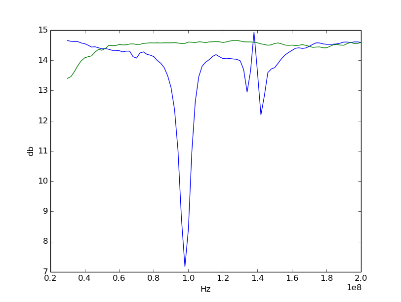
Green - No Filter
Blue - Low-Pass Filter[/caption]