You've Reached the Center of the Internet
It's a blog
Expected Outs Difference -- A simple team fielding metric
In this post, I’m going to outline a simple baseball team fielding metric I thought of. I’m calling it Expected Outs Difference or EOD.
Here’s the plan:
- Obtain a data set of balls put in play
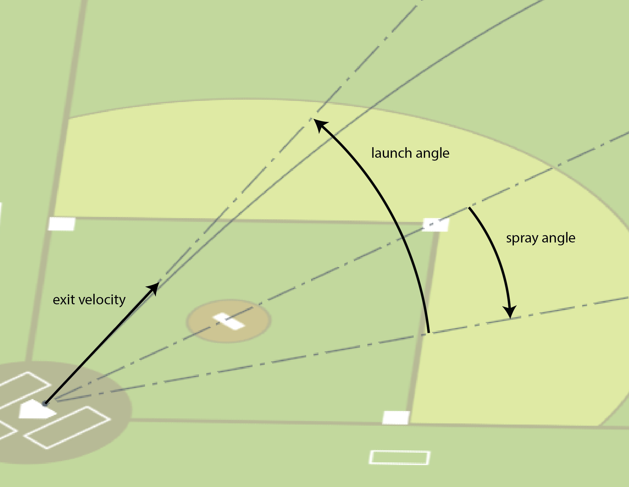
- Train a supervised model to predict whether a given ball will become and out based on exit velocity, launch angle, and spray angle
- Evaluate a team’s defense by running the model against each ball they faced and comparing the predicted outs with the actual ones
This method allows me to compare how well a team’s defense does at compared to what we’d expect based on how other teams do.
The data
I started by downloading a 2023 Statcast dataset using pybaseball. This gave me a table containing every pitch from the season.
from pybaseball import statcast
from pybaseball.datahelpers.statcast_utils import add_spray_angle

OUTS_EVENTS = ["field_out", "fielders_choice_out", "force_out", "grounded_into_double_play", "sac_fly_double_play", "triple_play", "double_play"]
START_DATE = "2023-03-01"
END_DATE = "2023-10-01"

data = add_spray_anglestatcast(start_dt=START_DATE, end_dt=END_DATE))

# filter out strikes and balls
balls_in_play = data[data["type"] == "X"]

# filter out foul outs
balls_in_play = balls_in_play[balls_in_play["spray_angle"].between(-45, 45)]

# label outs
balls_in_play["out"] = balls_in_play["events"].isin(OUTS_EVENTS)

# drop rows with missing data
balls_in_play = balls_in_play.dropna(subset=["launch_angle", "launch_speed", "spray_angle"])
Statcast provides a lot of information, but what I most cared about was exit velocity, launch angle, spray angle, and play outcome.
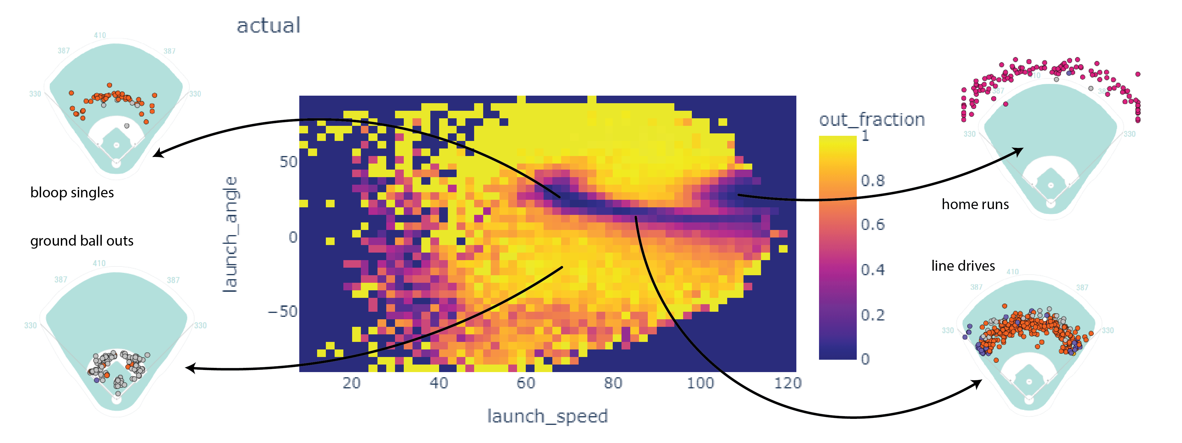
Here’s a 2D histogram showing the fraction of the hits within bins in exit velocity and launch angle that became outs.
Balls in the dark areas usually fall for hits.
Balls in the yellow areas are usually outs.
The model
I trained an SKLearn KNeighbors classifier. To make a prediction, this model looks up the eight most similar hits. If most of those hits became outs, the model classifies it as an out. If not, the model classifies it as a non-out.
from sklearn.neighbors import KNeighborsClassifier

X = balls_in_play[["launch_speed", "launch_angle", "spray_angle"]]
y = balls_in_play["out"]
clf = KNeighborsClassifier(n_neighbors=8).fit(X, y)

balls_in_play["predicted_out"] = clf.predict(X)
This isn’t perfect. When the model is classifying a point, it will always find the point itself as one of the nearest neighbors. I don’t think this is a big issue though.
Calculating EOD
Finally, I used the model to evaluate Expected Outs Difference.
# create a column giving the id of the fielding team
balls_in_play["fielding_team"] = np.where(balls_in_play["inning_topbot"] == "Top", balls_in_play["home_team"], balls_in_play["away_team"])

# group by fielding team and sum outs and predicted outs
teams = balls_in_play.groupby("fielding_team").agg({"out": "sum", "predicted_out": "sum", "events": "count"})

# subtracting the expected outs from the predicted outs gives Expected Outs Difference
teams["out_diff"] = teams["out"] - teams["predicted_out"]
teams.sort_values("out_diff", ascending=False)
              out	   predicted_out    events      out_diff
fielding_team
MIL           2634          2561          3947          73
CHC           2622          2578          4057          44
BAL           2719          2679          4183          40
AZ            2787          2754          4309          33
TEX           2658          2626          4072          32
TOR           2702          2672          4204          30
SEA           2609          2580          3989          29
LAD           2729          2704          4144          25
CLE           2751          2730          4231          21
ATL           2581          2566          4035          15
KC            2688          2677          4272          11
SD            2565          2558          3919          7
DET           2783          2781          4310          2
CWS           2541          2539          4002          2
PIT           2766          2764          4350          2
MIN           2673          2677          4121          -4
NYM           2610          2619          4088          -9
NYY           2771          2780          4237          -9
TB            2719          2735          4146          -16
SF            2661          2681          4178          -20
WSH           2731          2754          4367          -23
MIA           2645          2669          4139          -24
HOU           2623          2649          4061          -26
OAK           2635          2667          4234          -32
STL           2922          2962          4660          -40
PHI           2772          2821          4301          -49
LAA           2620          2685          4153          -65
BOS           2633          2698          4179          -65
CIN           2636          2717          4179          -81
COL           2864          2957          4662          -93
Evaluating EOD against other fielding metrics
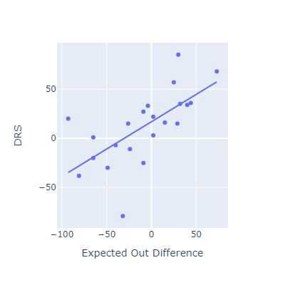
This approach seems to roughly match other popular fielding metrics.
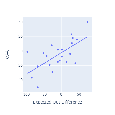
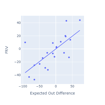
I think my method here is most conceptually similar to OAA. Oddly, that’s the metric that EOD correlates most poorly with.