Deriving FIP -- Fielding Independent Pitching

If you’re a baseball fan, you’ll probably have come across a stat called FIP or Fielding Independent Pitching. As I understand it, FIP was designed by Tom Tango to track a pitcher’s peformance in a way that doesn’t depend on fielders or on which balls happen to fall between them or get caught. Because it removes these factors that are outside of a pitcher’s control, FIP is also said to me more stable year-to-year and to be a better measure of a pitcher’s skill.

I believe the theory behind this comes from work by Voros McCracken showing that pitchers don’t have much control over the fraction of balls put in play that fall for hits. This conflicts with some baseball common sense ideas like “pitching to contact”, but let’s leave that aside for now. The fraction of balls in play that become hits is sometimes called BABIP or Batting Average on Balls In Play. By diminishing the luck-based effects of BABIP, one can build a pitching statistic that’s more indicative of a pitcher’s true ability. That’s the idea.

To accomplish this goal, FIP is based on results that pitchers have the most control over: home runs, strikeouts, walks, and hit by pitch. Also, it’s constructed to have a similar scale to ERA to make it familiar to fans. Until recently, that was about all I knew.

It’s easy to find a formula online:

where \(\mathrm{HR}\), \(\mathrm{BB}\), \(\mathrm{HBP}\), \(\mathrm{SO}\), and \(\mathrm{IP}\) are the number of home runs, walks, hit by pitch, strike outs, and innings pitched collected by the pitcher, respectively. \(C_{\mathrm{FIP}}\) is a constant which varies year by year and is apparently usually around three. The constant brings FIP into the same range as ERA.

But where do the 13, 3, -2, and constant come from though? This is a bit harder to find.

In this post, I’ll derive a version of FIP in a way that makes sense to me. I’ll touch on this at the end, but I don’t think this is the way it’s actually done.

My method is simple: I trained a linear regression model to predict a pitcher’s ERA based on \(\mathrm{HR}\), \(\mathrm{BB} + \mathrm{HBP}\) and \(\mathrm{SO}\). FIP is just a linear combination of those parameters, so it will be easy to compare the trained parameters of the linear model with the real formula.

A look at the data

I used pybaseball to download full season pitching data from 2015 to 2023.

The relationships between the raw statistics are as you’d expect. For example, here’s ERA plotted against HR and SO: 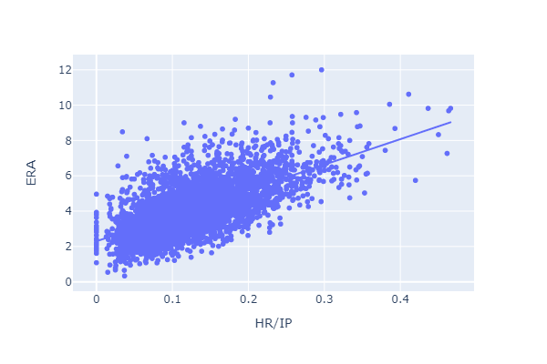Home runs allowed per inning pitched has a positive relationship with ERA.

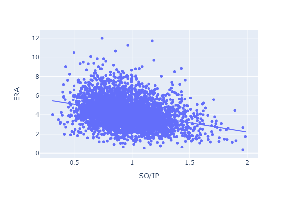Strikeouts per inning has a negative relationship with ERA. Let’s move on.

Training a linear model

Training a linear model is pretty easy:

from pybaseball import pitching_stats
from sklearn.linear_model import LinearRegression

logs = pitching_stats(2021, 2023, qual=25)

logs["UBB"] = logs["BB"] - logs["IBB"] # unintentional walks is total walks minus intentional walks
logs["UBB_HBP"] = logs["UBB"] + logs["HBP"] # sum walks and hit by pitch

X = logs[["HR", "UBB_HBP", "SO"]].div(logs["IP"], axis=0) # normalize by innings pitched
y = logs["ERA"]
weight = logs["IP"]
fip_reg = LinearRegression().fit(X, y, sample_weight=weight)

Two things to point out here:

1. I excluded pitchers with less than 25 innings pitched using the qual kwarg in the pitching_stats() call.
2. I weighted the samples based on innings pitched using sample_weight.

The relationship between ERA and FIP looks reasonable:

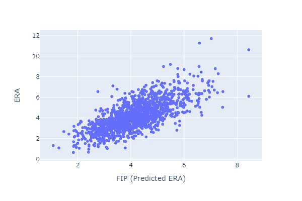
Here are the fitted parameters:

fip_reg.coef_, fip_reg.intercept_
> (array([13.28482645,  3.2804091 , -1.78295967]), 2.8140810888761045)

So my version of FIP is

vs the regular version

Maybe this is silly, but I was a little shocked at how closely they align. If you round my coefficients to the nearest whole number, the equations are identical.

Does FIP work?

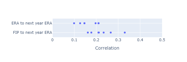
If FIP works as intended, it should have more year-to-year predictive power than ERA. I calculated the correlation between ERA in one year and ERA in the next year with the correlation between FIP in one year and ERA in the next year. I’m comparing

with

Based on year to year correlations from 2015 to 2023, FIP does seem to have better year-to-year predictive power. The plot below shows a 1D scatter plot of the year-to-next-year correlations from 2015 to 2023.

xFIP

If you’ve seen FIP, you may also have come across a related stat called xFIP (the x stands for “expected”). It’s based on a familiar observation. Just like pitchers seem to not have much control over BABIP, they also don’t seem to have much control over their home run to fly ball ratio. xFIP is just like FIP except that it replaces the player’s actual home run total with an expected home run total by replacing their home run to fly ball ratio with the league average ratio:

with

This has always felt a little strange to me. Now xFIP is back to being dependent on fielders and the luck of precisely where balls land.

It’s simple to implement:

league_avg_hr_fb = logs["HR"].div(logs["FB"]).mean()
logs["xHR"] = logs["FB"] * league_avg_hr_fb

X = logs[["xHR", "UBB_HBP", "SO"]].div(logs["IP"], axis=0) # normalize by innings pitched
y = logs["ERA"]
weight = logs["IP"]
xfip_reg = LinearRegression().fit(X, y, sample_weight=weight)

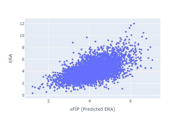
The relationship between (same year) xFIP and ERA seems worse than that between FIP and ERA:

Does xFIP work?

I repeated the above experiments to look at xFIP’s predictive power. 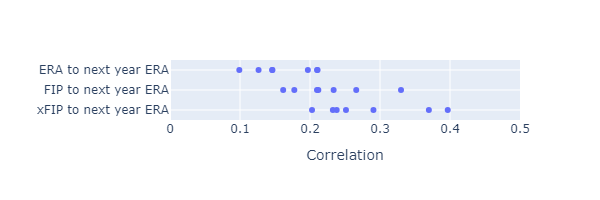xFIP seems to have somewhat more predictive power than FIP or ERA.

How similar is this to real FIP?

At time of writing, I haven’t found a satisfying derivation of the FIP equation. As best I can tell, the coefficients are derived from a type of run value estimate of each possible plate appearance outcome called linear weights. That topic probably deserves a post of its own. However, my method found an equation that’s very similar to the real FIP equation, so maybe it doesn’t matter how it was originally calculated. If two different methods arrive at the same answer, that ought to give us extra confidence in the result.