Optimizing Steering Car Paths with PyTorch

Want to see another bizarre way to use PyTorch? If you've read some of my recent posts, you've seen the basic idea before. I'm using automatic differentiation and gradient descent, this time to optimize the path of a car. The model is similar to a Reeds-Shepp car, a simple steering car model. The state at time step \(i\) is defined by a 2D position and an angle, \((x_i, y_i, \theta_i)\). In each step of the simulation, the car's state is updated based on an input consisting of speed and steering angle \((v_i, \phi_i)\).

\(x_{i+1} = x_i + v_i \cos{\theta_i} dt\)
\(y_{i+1} = y_i + v_i \sin{\theta_i} dt\)
\(\theta_{i+1} = \theta_i + v_i \phi_i dt\)

I simulated the car for \(n_\text{steps}\) steps, with a target position and angle, \((x_t, y_t, \theta_t)\) and a cost function, \(c\), which depended on the distance from the target position and the distance from the target angle in the final step.

\(c= \left(\theta_t - \theta_n\right)^2 +\left(x_t - x_n\right)^2 + \left(y_t - y_n\right)^2 \)

I used automatic differentiation to find the derivates \(\frac{dc}{dv_i}\) and \(\frac{dc}{d\phi_i}\), which I used to update the inputs.

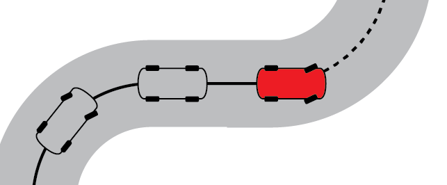
Check out some results. The animated plot below shows an example optimization, with the working solution evolving over time. The car starts at \((0,0)\), facing right and its target is \((3,3)\), facing down. The starting position and direction are represented by the red arrow and the target position and direction are represented by the green arrow.

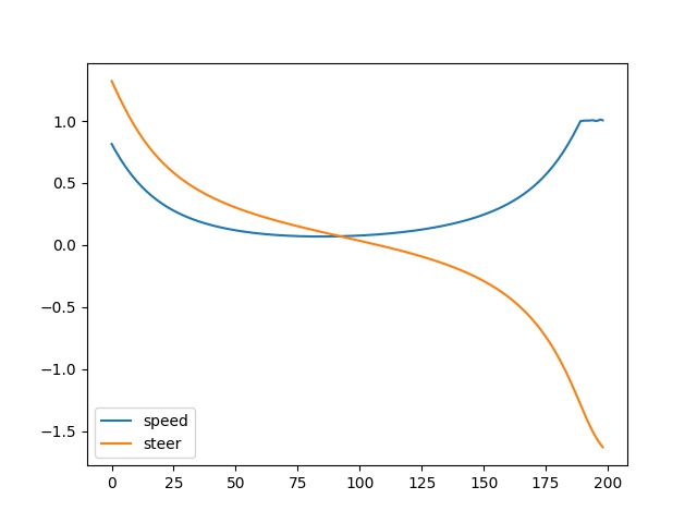
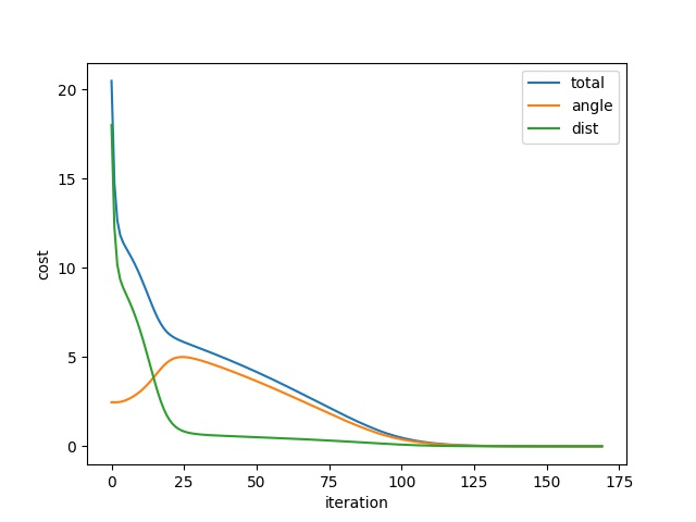
In the first frame of the animation, the inputs are initialized to zero and the car does not move. In the ultimate solution, the car performs a wide left turn into its final position. The plots below shows the input that produced that trajectory and the evolution of the cost function.

Code below.

import torch
import numpy as np
import matplotlib.pyplot as plt
from scipy import optimize

n_steps = 200 # number of steps to test the car performance
speeds = torch.zeros(n_steps-1, requires_grad=True) # init speed control tensor
steers = torch.zeros(n_steps-1, requires_grad=True) # init steering control tensir
dt = .1 # time step for dynamics

target_pos = torch.tensor([3.,3.]) # target position for the car
target_angle = torch.tensor(3*np.pi/2.) # target angle for the car

# finds the trajectory from the speed and steering commands
def test_car(speeds, steers):
    angles =[torch.tensor(0.)]
    xs = [torch.tensor(0.)]
    ys = [torch.tensor(0.)]

    # simulate the car performance
    for i in range(1,n_steps):
        speed =  torch.clamp(speeds[i-1], -1., 1.) # limit the speed
        steer = torch.clamp(steers[i-1], -10., 10.) # limit the steering angle
        xs.append(xs[-1]+ dt * speed * torch.cos(angles[-1]))
        ys.append(ys[-1]+ dt * speed * torch.sin(angles[-1]))
        angles.append((angles[i-1] + dt * speed * steer)%(2*np.pi))
    return xs, ys, angles


# list to keep track of objective progress
costs = []
angle_costs = []
dist_costs = []

# cost plot
fig_cost = plt.figure()
ax_cost = fig_cost.add_subplot(111)
ax_cost.autoscale(enable=True, axis="y", tight=False)
ax_cost.set_xlabel("iteration")
ax_cost.set_ylabel("cost")

li_cost, = ax_cost.plot([],[])
li_cost_ang, = ax_cost.plot([],[])
li_cost_dist, = ax_cost.plot([],[])

# input plot
fig_in = plt.figure()
ax_in = fig_in.add_subplot(111)
ax_in.autoscale(enable=True, axis="y", tight=False)

li_speed, = ax_in.plot(speeds.detach().numpy())
li_steer, = ax_in.plot(steers.detach().numpy())

# trajectory plot
fig_traj = plt.figure()
ax_traj = fig_traj.add_subplot(111)

li_traj, = ax_traj.plot([])
l = 0.25
ax_traj.arrow(0,0,0,l, width=0.05, color="red")
ax_traj.arrow(*target_pos, l* torch.cos(target_angle), l*torch.sin(target_angle), width=0.05, color="green")
ax_traj.set_xlim(-1.,4.)
ax_traj.set_ylim(-1.,4.)

fig_cost.canvas.draw()
fig_traj.canvas.draw()
fig_in.canvas.draw()
plt.show(block=False)

optimizer =  torch.optim.SGD([speeds, steers], lr=0.1)
#optimizer =  torch.optim.Adam([speeds, steers])

for i in range(170):
    # run simulation
    xs, ys, angles = test_car(speeds, steers)

    # calculate costs
    angle_error = target_angle - angles[-1]
    angle_cost = torch.min(torch.min((angle_error+2*np.pi)**2, (angle_error-2*np.pi)**2), angle_error**2)

    dist_cost = (target_pos[0] - xs[-1])**2 + (target_pos[1] - ys[-1])**2   

    cost = dist_cost + angle_cost

    # save costs
    costs.append(cost)
    angle_costs.append(angle_cost)
    dist_costs.append(dist_cost)

    #calculate gradients
    optimizer.zero_grad()
    cost.backward()

    # update inputs
    optimizer.step()

    # update plots
    li_cost.set_data(range(len(costs)),costs)
    li_cost_ang.set_data(range(len(angle_costs)),angle_costs)
    li_cost_dist.set_data(range(len(dist_costs)),dist_costs)
    li_speed.set_ydata(speeds.detach().numpy())
    li_steer.set_ydata(steers.detach().numpy())
    li_traj.set_data(xs, ys)
    
    ax_cost.relim()
    ax_cost.autoscale_view()
    ax_cost.legend(["total", "angle", "dist"])

    ax_in.relim()
    ax_in.autoscale_view()
    ax_in.legend(["speed", "steer"])

    fig_traj.canvas.draw()
    fig_cost.canvas.draw()
    fig_in.canvas.draw()

You've Reached the Center of the Internet

It's a blog

Optimizing Steering Car Paths with PyTorch